Gibbs Sampling Algorithm

import numpy as np
import scipy as sp
import matplotlib.pyplot as plt

plt.style.use("fivethirtyeight")

The Gibbs sampler is a special case of the Metropolis sampler in which the proposal distributions exactly match the posterior conditional distributions and naturally proposals are accepted 100% of the time.

However a specialty of Gibbs Sampler is that can allow one to estimate multiple parameters.

In this section, we will use Normal-Normal and Gamma-Normal conjugate priors to demonstrate the algorithm of Gibbs sampler.

Suppose you want to know the average height of female in your city, in the current setting, we assume \(\mu\) and \(\tau\) are our parameters of interest for estimation. Note that in conjugate prior section we assumed \(\tau\) to be known, however in Gibbs sampling, both can be estimated.

A prior of normal distribution will be assumed for \(\mu\) with hyperparameters \[ \text{inverse of }\sigma_0:\tau_0 = .35\\ \text{mean}:\mu_0 = 170 \]

A prior of gamma distribution will be assumed for \(\tau\) since it can’t be negative. \[ \text{shape}: \alpha_0 = 2\\ \text{rate}:\beta_0 = 1 \]

The priors graphically are

mu_0, tau_0 = 170, 0.35
x_mu = np.linspace(150, 190, 100)
y_mu = sp.stats.norm(loc=mu_0, scale=1 / tau_0).pdf(x_mu)

alpha_0, beta_0 = 2, 1
x_tau = np.linspace(0, 8, 100)
y_tau = sp.stats.gamma(a=alpha_0, scale=1 / beta_0).pdf(x_tau)

fig, ax = plt.subplots(figsize=(15, 5), nrows=1, ncols=2)
ax[0].plot(x_mu, y_mu, label=r"$\mu_0={}, \tau_0={}$".format(mu_0, tau_0))
ax[0].set_title(r"Prior of $\mu$")
ax[0].legend()
ax[1].plot(x_tau, y_tau, label=r"$\alpha_0={}, \beta_0={}$".format(alpha_0, beta_0))
ax[1].set_title(r"Prior of $\tau$")
ax[1].legend()
plt.show()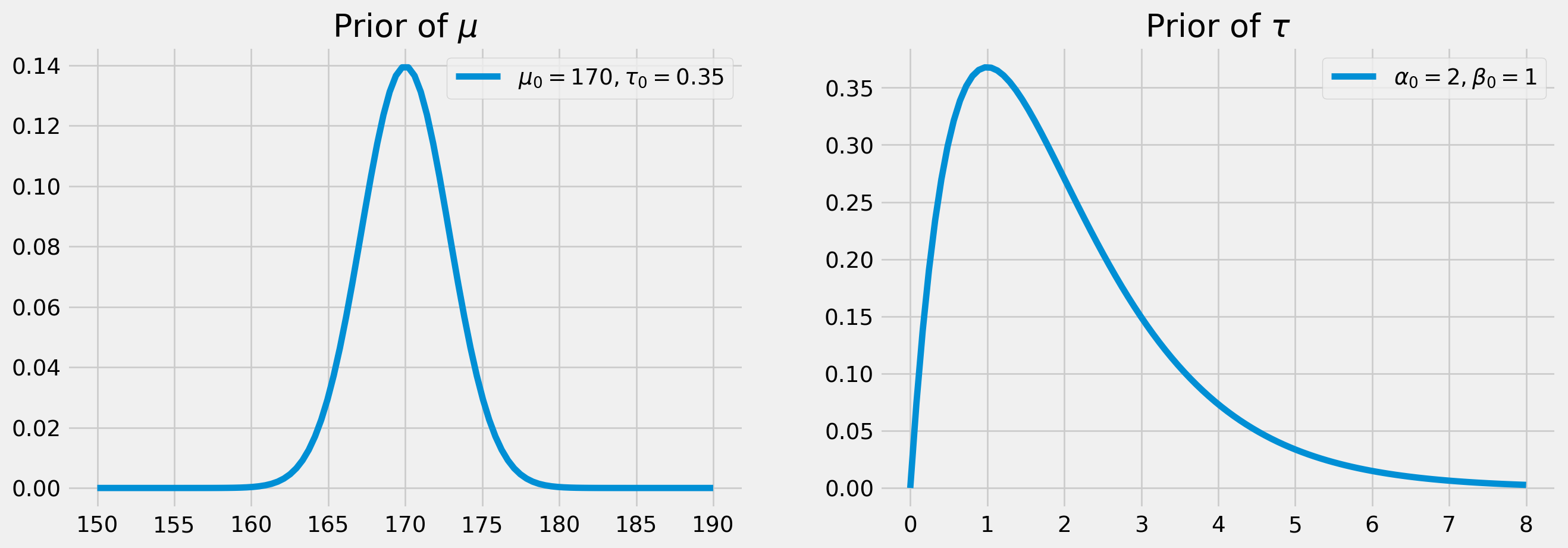

Here is the joint frequency distribution of \(\mu\) and \(\tau\).

n = 30000
mu_height = sp.stats.norm(loc=mu_0, scale=1 / tau_0).rvs(n)
tau_height = sp.stats.gamma(a=alpha_0, scale=1 / beta_0).rvs(n)
fig, ax = plt.subplots(figsize=(8, 5))
ax.scatter(mu_height, tau_height, s=3)
plt.show()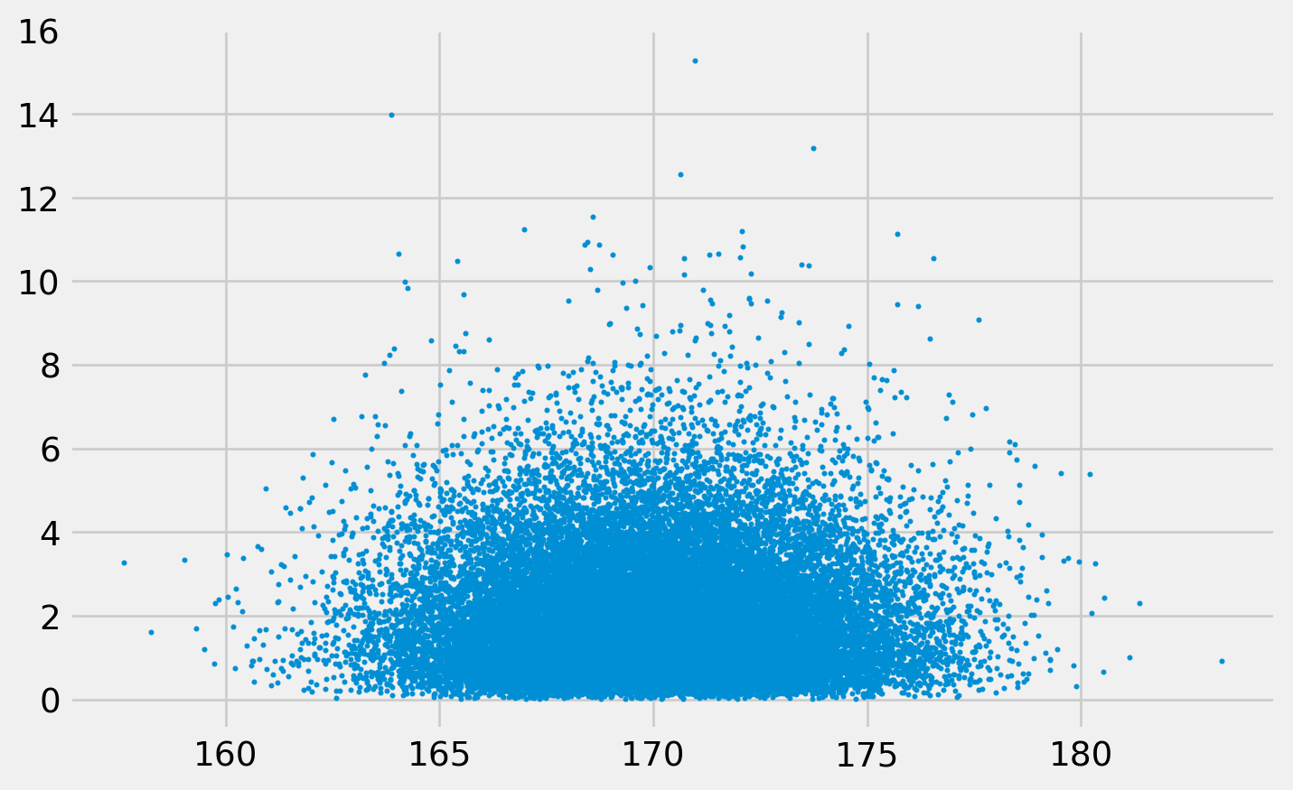

Choose an initial value of proposal of \(\tau\), denoted as \(\tau_{\text{proposal},0}\), the \(0\) subscript represents the time period, since this is the initial value.

Say \[ \tau_{\text{proposal},0} = 7 \]

Next step is to obtain \[ \mu_{\text{proposal},0}|\tau_{\text{proposal},0} \] where \(\mu_{\text{proposal},0}\) is the first value of proposal \(\mu\) conditional on \(\tau_{\text{proposal},0}\).

Now go collect some data, for instance you measured \(10\) random women’s heights, here’s the data.

heights = np.array([156, 167, 178, 182, 169, 174, 175, 164, 181, 170])
np.sum(heights)

1716

Recall we have a sets of analytical solutions on Normal-Normal conjugate derived in chapter 2

\[\begin{align} \mu_{\text {posterior }} &=\frac{\tau_{0} \mu_{0}+\tau \sum x_{i}}{\tau_{0}+n \tau}\\ \tau_{\text {posterior }} &=\tau_{0}+n \tau \end{align}\]

Substitute \(\tau_{\text{proposal},0}\) into both formula.

\[ \mu_{\text {posterior},1} =\frac{\tau_{0} \mu_{0}+\tau_{\text{proposal},0} \sum_{i=0}^{100} x_{i}}{\tau_{0}+n \tau_{\text{proposal},0}}=\frac{.15\times170+7\times 1716}{.15+10\times7}\\ \tau_{\text {posterior}, 1} =\tau_{0}+n \tau_{\text{proposal},0} = .15 + 10\times 7 \]

mu_post = [0]
tau_post = [0]  # 0 is placeholder, there isn't 0th eletment, according to algo

tau_proposal = [7]
mu_proposal = [0]  # 0 is placeholder

mu_post.append((0.15 * 170 + tau_proposal[0] * 1716) / (0.15 + 10 * tau_proposal[0]))
tau_post.append(0.15 + 10 * tau_proposal[0])

Draw a proposal from updated distribution for \(\mu\), that is \(\mu_{\text{posterior}, 1}\) and \(\tau_{\text{posterior}, 1}\)

mu_proposal_draw = sp.stats.norm(loc=mu_post[1], scale=1 / tau_post[1]).rvs()
mu_proposal.append(mu_proposal_draw)

Now turn to \(\tau\) for a proposal, there is also Gamma-Normal conjugate prior which we didn’t derive before. But here are the posterior \[\begin{align} \alpha_{\text{posterior}}&=\alpha_0+\frac{n}{2}\\ \beta_{\text{posterior}}&=\beta_0+\frac{\sum_{i=1}^{n}\left(x_{i}-\mu\right)^{2}}{2} \end{align}\]

alpha_post = [0]
beta_post = [0]

alpha_post.append(alpha_0 + 10 / 2)
beta_post.append(beta_0 + np.sum((heights - mu_post[-1]) ** 2) / 2)

tau_proposal_draw = sp.stats.gamma(a=alpha_post[-1], scale=1 / beta_post[-1]).rvs()
tau_proposal.append(tau_proposal_draw)

tau_proposal

[7, 0.025437814559547613]

Gibbs Sampling in a Loop

mu_post, tau_post, alpha_post, beta_post, mu_proposal, chain_size = (
    [],
    [],
    [],
    [],
    [],
    10000,
)


def gibbs_norm_gam_joint(
    mu_0=170,
    tau_0=0.35,
    tau_proposal_init=7,
    alpha_0=2,
    beta_0=1,
    chain_size=chain_size,
    data=heights,
):
    tau_proposal = [tau_proposal_init]
    n = len(data)
    for i in range(chain_size):

        mu_post.append(
            (tau_0 * mu_0 + tau_proposal[-1] * np.sum(data))
            / (tau_0 + n * tau_proposal[-1])
        )
        tau_post.append(tau_0 + n * tau_proposal[-1])

        mu_proposal_draw = sp.stats.norm(loc=mu_post[-1], scale=1 / tau_post[-1]).rvs()
        mu_proposal.append(mu_proposal_draw)

        alpha_post.append(alpha_0 + n / 2)
        beta_post.append(beta_0 + np.sum((heights - mu_post[-1]) ** 2) / 2)

        tau_proposal_draw = sp.stats.gamma(
            a=alpha_post[-1], scale=1 / beta_post[-1]
        ).rvs()
        tau_proposal.append(tau_proposal_draw)
    return mu_post, tau_post

mu_post, tau_post = gibbs_norm_gam_joint()

Calculate the moment matching PDF for both distributions.

x_mu = np.linspace(170, 172.2, 100)
mu_dist = sp.stats.norm(loc=np.mean(mu_post), scale=np.std(mu_post)).pdf(x_mu)

To acquire \(\alpha\) and \(\beta\), we need solve a system of equations \[ \mu=\frac{\alpha}{\beta}\\ \sigma^2=\frac{\alpha}{\beta^2} \]

from scipy.optimize import fsolve


def solve_equ(x, mu=np.mean(tau_post), sigma=np.std(tau_post)):
    a, b = x[0], x[1]
    F = np.empty(2)
    F[0] = mu - x[0] / x[1]
    F[1] = sigma**2 - x[0] / (x[1] ** 2)
    return F


xGuess = np.array([2, 2])
z = fsolve(solve_equ, xGuess)
print("alpha: {}".format(z[0]))
print("beta: {}".format(z[1]))

alpha: 0.7078335859779051
beta: 1.1964149217042301

x_tau = np.linspace(0.37, 1, 100)
tau_dist = sp.stats.gamma(a=z[0], scale=1 / z[1]).pdf(x_tau)

fig, ax = plt.subplots(figsize=(18, 12), nrows=2, ncols=2)
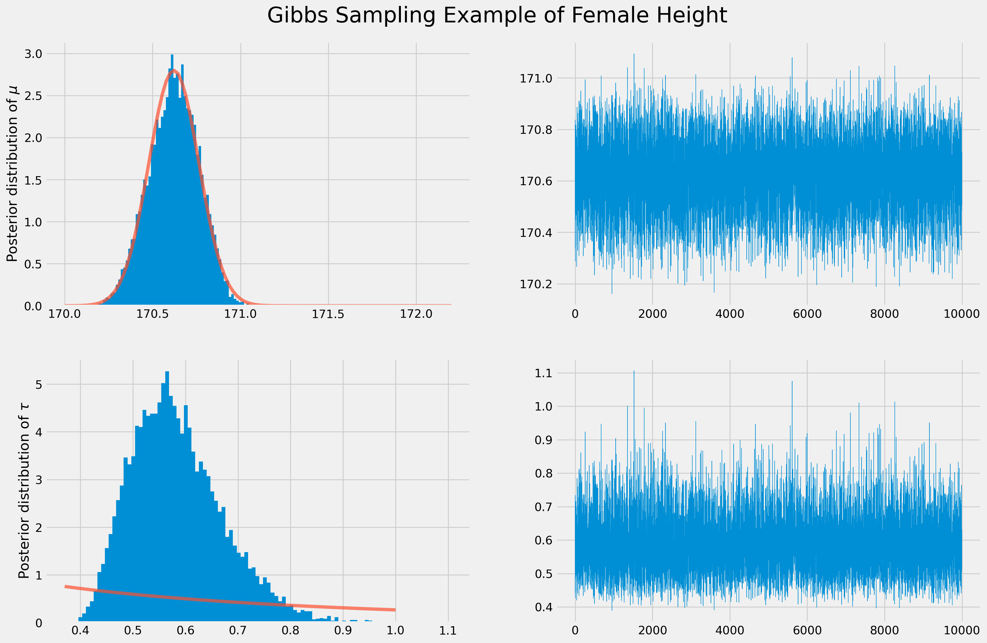
ax[0, 0].hist(mu_post, bins=100, density=True)
ax[0, 0].plot(x_mu, mu_dist, alpha=0.7)
ax[0, 0].set_ylabel("Posterior distribution of $\mu$")
ax[1, 0].hist(tau_post[1:], bins=100, density=True)
ax[1, 0].plot(x_tau, tau_dist, alpha=0.7)
ax[1, 0].set_ylabel(r"Posterior distribution of $\tau$")
ax[0, 1].plot(np.arange(chain_size - 1), mu_post[1:], lw=0.5)
ax[1, 1].plot(np.arange(chain_size - 1), tau_post[1:], lw=0.5)
fig.suptitle("Gibbs Sampling Example of Female Height", y=0.93, size=26)
plt.show()

<>:4: SyntaxWarning:

invalid escape sequence '\m'

<>:4: SyntaxWarning:

invalid escape sequence '\m'

/tmp/ipykernel_3551/2211377782.py:4: SyntaxWarning:

invalid escape sequence '\m'